IMPROVING LIVES THROUGH DATA ECOSYSTEMS

In April and May 2022 Stats SA is updating its seasonal adjustment models for monthly business cycle indicators, namely mining, manufacturing, electricity, building, wholesale, retail, motor, tourist accommodation, food & beverages, land transport, and civil cases for debt.

What is seasonal adjustment, and why is it so important for measuring and analysing the economy? We explore these questions using three examples – retail trade, manufacturing, and electricity consumption.

Retail trade

A good place to start our journey is retail trade. This is because there is a seasonal effect in retail that is strong and familiar, with sharply higher sales in November and December brought about by the festive season. The pattern is clearly visible in Figure 1. Typically we see high sales in November as some people get their Christmas shopping done early and many others take advantage of Black Friday promotions. December sales are even higher.

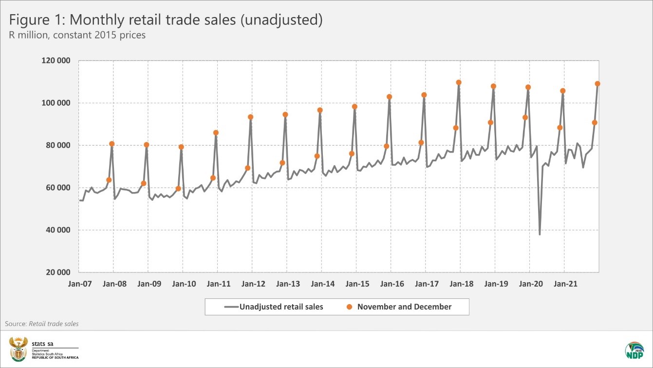
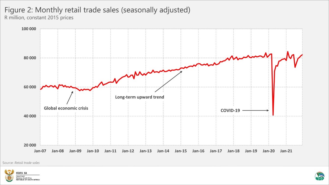
While the month-to-month patterns in retail sales are interesting and of great importance for retailers in planning their purchases and inventories, the spikes in the graph make trends in the data quite difficult to follow. This is where seasonal adjustment comes in. Because the seasonal pattern in the unadjusted series is so clear and regular, we can estimate the seasonal effects and remove them, leaving us with a seasonally adjusted series.

The seasonally adjusted series for retail sales is shown in Figure 2, in which it is immediately easier to spot the global economic crisis of 2008–2009 and the long-term upward trend thereafter. Even the COVID-19 downward spike in April 2020 stands out more clearly. Note that seasonal adjustment removes the spikes that are clear and regular, not those which are caused by unusual circumstances such as a pandemic.

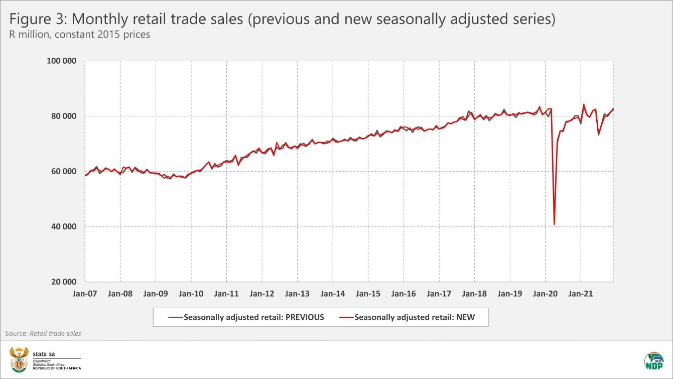
As more data points are added to a series, we learn a little more about its behaviour. The seasonally adjusted values for monthly business cycle indicators are revised each month, and from time to time the seasonal adjustment models (or programs) need to be re-estimated as well. The new model for retail trade produces results that are very close to the previous model, and this is generally the outcome that we see in the other indicators as well. Nevertheless, it is important to update the models because seasonal patterns can change over time. For instance, Black Friday has become more important for retail trade in recent years, and if you refer back to Figure 1 you will see that the November data points are clearly more elevated (compared with October) in the later years than in the earlier years. In other words the retail seasonal effect in November has strengthened over time, and our seasonal adjustment modelling has to capture that change. The previous and new seasonally adjusted series are compared in Figure 3.

Manufacturing production

The strongest months for manufacturing production are October and November, because the manufacturers are of course well aware that Black Friday and Christmas are coming. After a flurry of manufacturing activity in October and November, December and January tend to be subdued; February manufacturing is also quite subdued (it’s a short month), as is April (Easter and Freedom Day). Figure 4 shows the unadjusted and seasonally adjusted series together. Note how the seasonally adjusted series is much smoother than the unadjusted series.

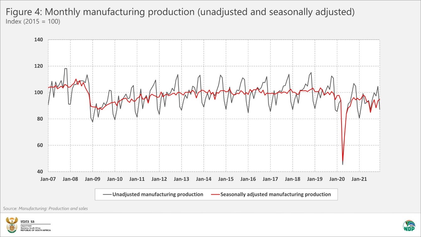
To further illustrate the importance of seasonal adjustment, let’s look at a specific month. In October 2019, manufacturing production grew by 10% compared with September 2019. That may sound like strong growth – 10% in a single month – but it is mostly seasonal. There is usually a big jump in production between September and October. When the seasonal effect is removed, we calculate from the seasonally adjusted series that production grew by only 2,4% between September and October 2019. For economists who monitor and analyse each new data point to assess how the economy is performing, monthly changes in seasonally adjusted series are a critical source of information.

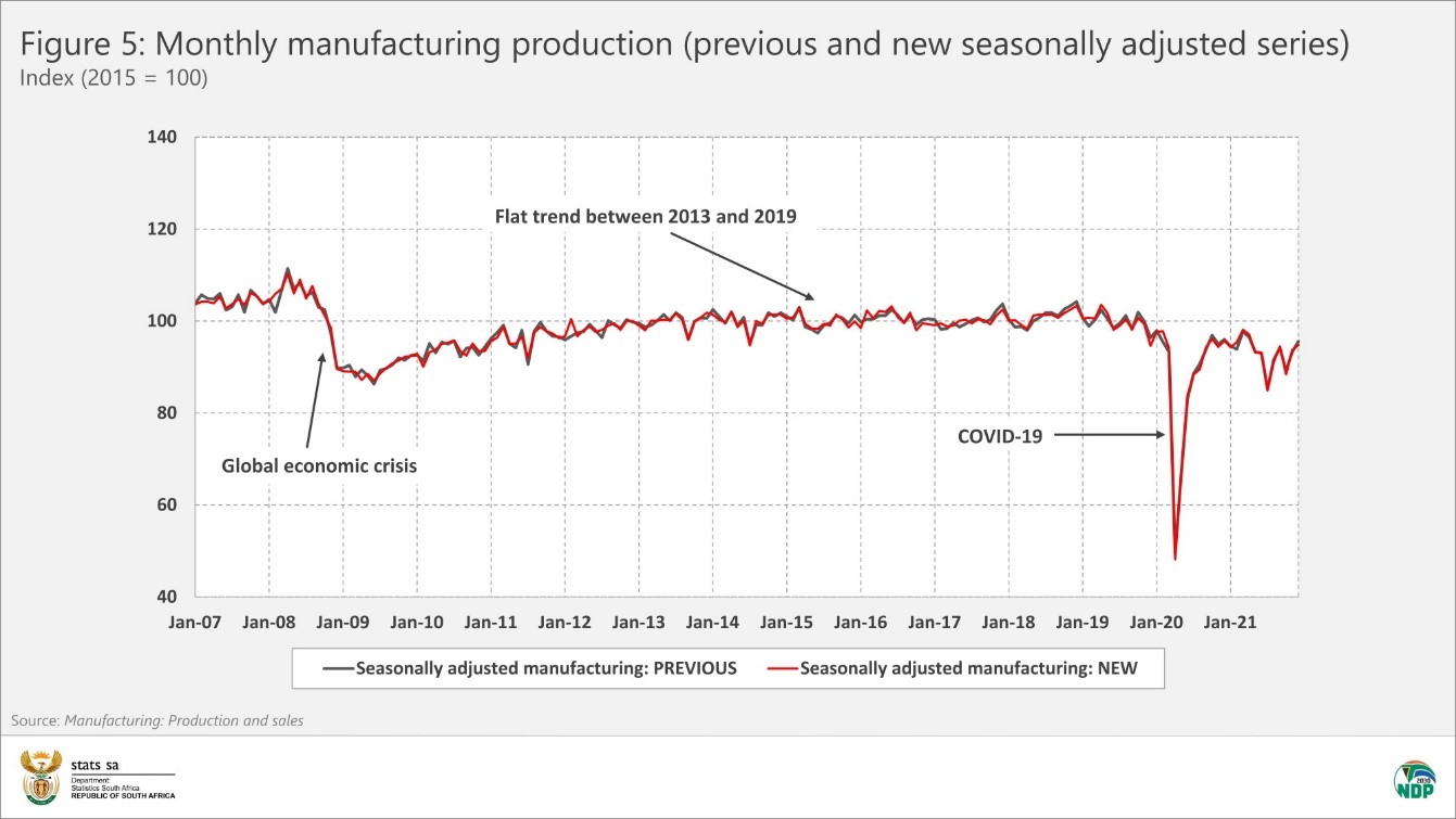
The previous and new seasonally adjusted series for manufacturing production are compared in Figure 5. The results are generally close. Greater differences are evident when comparing some of the components of manufacturing, but even these tend to be small.

Electricity consumption

Another series with strong seasonality is electricity consumption, whose pattern is largely driven by the weather. There is much stronger demand for electricity in the winter months for heating, as shown in Figure 6, where we use a moving average and a shorter time scale to illustrate the seasonality clearly.

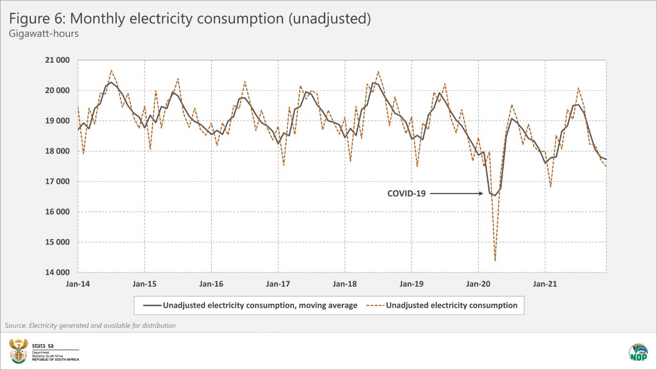
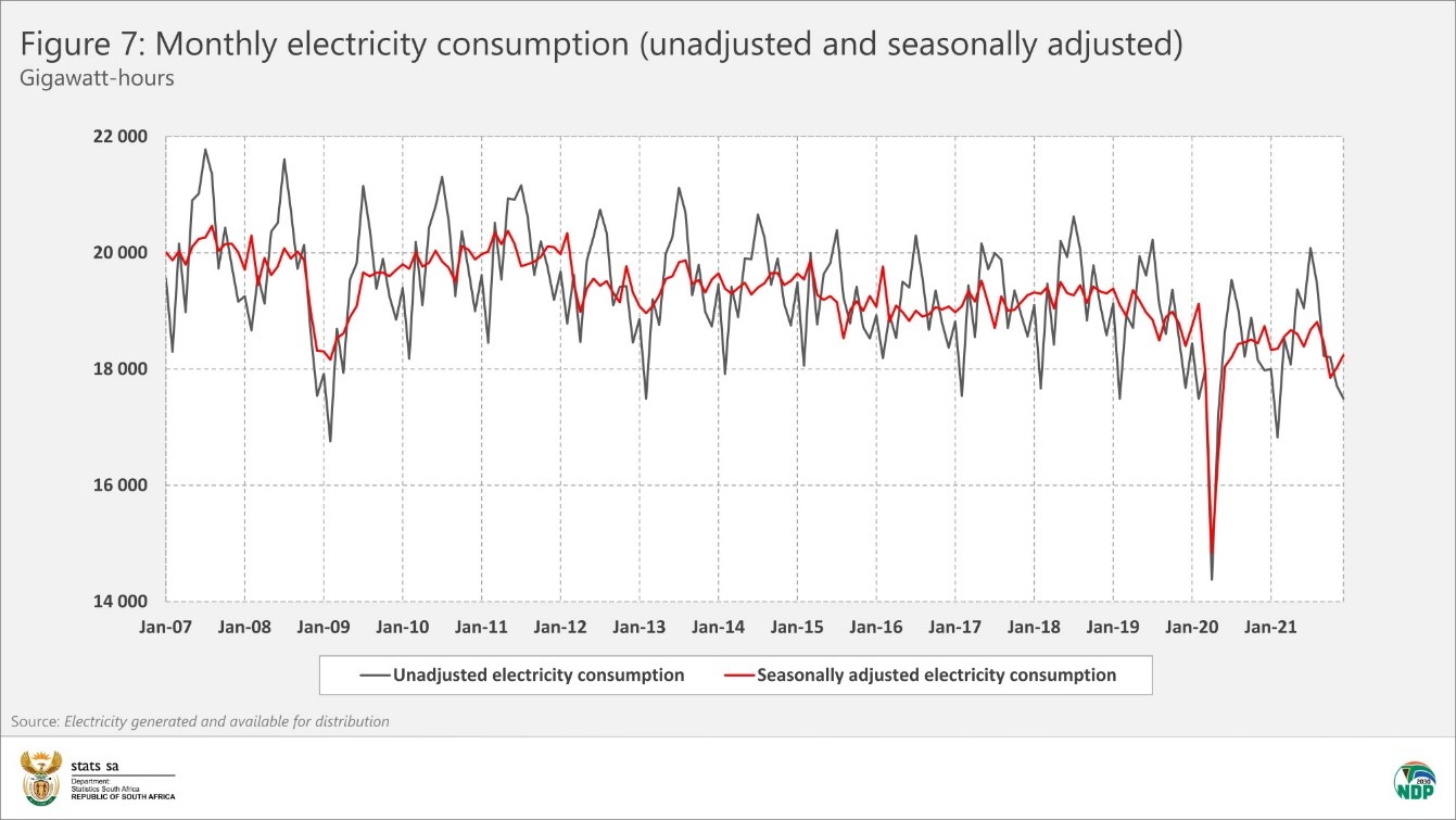
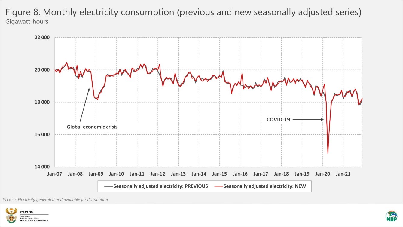
Figure 7 shows the unadjusted and seasonally adjusted electricity series together, and note once again how the seasonally adjusted series is much smoother than the unadjusted series. The previous and new seasonally adjusted series for electricity consumption are compared in Figure 8.

Simple in concept, complex in practice

The examples of retail, manufacturing and electricity illustrate that seasonal adjustment is an important technique for tracking trends in economic indicators and that the concept of seasonal adjustment is quite straightforward. However, the actual modelling of seasonally adjusted series is quite complex, and must take into account a variety of factors such as outliers, level shifts, transitory changes, and Easter, trading day, and length-of-month effects.

Outliers are unusually high or low values in the time series in particular months. A level shift is an abrupt but sustained change in the level of the time series. A transitory change refers to a series of outliers with temporary effects on the level of the series.

The Easter holidays may regularly affect economic activity before, during or after the holiday period. Unlike other public holidays which occur on the same date each year, the dates for Easter are not fixed and may occur in March or April. Such an effect, if it is present, is known as the Easter effect.

A trading day effect takes into account the composition of the calendar. For example, different months have different numbers of working days, and the number of specific days of the week can occur in differing frequency in the same month in different years. Days of the week can have different levels of activity, e.g. high retail sales on Saturdays. A length-of-month effect arises from the fact that some months are longer than others, i.e. 28, 29, 30 or 31 days.

Stats SA uses the X-12 ARIMA seasonal adjustment program developed by the United States Census Bureau. The program incorporates the elements mentioned above to create seasonally adjusted time series.

Where do I find out more?

Each of Stats SA’s monthly statistical releases with seasonal adjustment provides a link where users can find the specifications (metadata) for individual seasonal adjustment programs. For example, for the series discussed above, methodological notes are available for retail trade (download here), manufacturing (download here) and electricity (download here). Notes for other series will be published in due course. Keep track of our published statistical releases here.

Similar articles are available on the Stats SA website and can be accessed here.

For a monthly overview of economic indicators and infographics, catch the latest edition of the Stats Biz newsletter here.